• last modification: January 2015

VolcFlow has been developped for the simulation of volcanic flows at the Laboratoire Magmas et Volcans, Clermont-Ferrand by Karim Kelfoun (karim.kelfoun @ uca.fr) and collaborators.

VolcFlow has been be used:

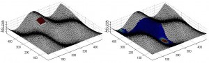
• for determining the rheological behaviour of dense pyroclastic flows and debris avalanches
• for visualizing deformations of the surface of debris avalanche and interpret or compare with field structures
• for volcanic hazard mapping
• for the the simulation of tsunami generated by volcanic flows
• for reproducing the emplacement of fluidized flows in laboratory
• for the simulation of lava flows
• for the simulation of dense and dilute pyroclastic flows

Simulation of Socompa avalanche, Kelfoun and Druitt, 2005

More than >200 users worldwide (in 2018)

2. The one-fluid version

The distributed version of VolcFlow is isothermal and simulates one fluid.
It has been used for the simulation of granular flows in laboratory, debris avalanches, lahars and dense pyroclastic flows.
Users can use predefined rheologies as weel as their own rheological laws compatible with the depth averaged approach.Sedimentation and erosion can be simulated too.

2.1 Simulation of debris avalanches

Simulation of Socompa debris avalanche (details on the natural deposits of Socompa avalanche).
See the movie file (7.7 Mo)
Read the following paper for further details:
Kelfoun K, Druitt TH (2005) Numerical modeling of the emplacement of Socompa rock avalanche, Chile . J Geophys Res 110 : B12202.1-12202.13 DOI:10.1029/2005JB003758

VolcFlow also allows to reconstruct strain ellipse and surface deformation of the flows (See the movie file, 2.1 Mo).
This may be very usefull to compare field structures of the natural deposits to numerical simulations.
Read the following paper for further details:
Kelfoun K, Druitt TH, van Wyk de Vries B, Guilbaud MN, Topographic reflexion of Socompa debris avalanche, Chile, Bull. Volcanol, 2008

2.2 Simulation of pyroclastic flows

The rheological behaviour of pyroclastic flows is very complex. VolcFlow can be used to estimate it, reproducing well known eruptions with different rheological laws and comparing numerical results to natural deposits.

Pyroclastic flows at Tungurahua volcano (more details on Tungurahua activity)
See the movie file (7 Mo)
Read the following paper for further details: Kelfoun K, Samaniego P, Palacios P, Barba D, 2009, Is frictional behaviour suitable for pyroclastic flow simulation: comparison with a well constrained eruption at Tungurahua volcano (Ecuador). Bulletin of Volcanology.

2.3 Hazard maps

It is possible to generate hasard maps with VolcFlow. The maps can be drawn either for one event or for several scenarios taking into account a range of volumes, column heights, etc…
Of course, this need the knowledge of the rheological behaviour of the simulated flows, which is the main problem to deal with.

An example of Hasard map of Guagua Pinchincha, Ecuador.
Hasard maps generated with VolcFlow at Guagua Pichincha (Ecuador) and Reventador (Ecuador, J. Bourquin)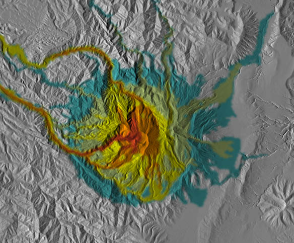

2.4 Erosion and sedimentation

VolcFlow can also take into account sedimentation and erosion during emplacement.

Example of a viscous body sedimenting with time
See the movie file (400 Ko)

You can add you own laws of sedimentation and erosion in the « source »-string.
For sedimentation, the mass and momentum conservation is simply achieved by changing the mass.
In erosion, the flow is slowed down, and you have to write the laws needed for momentum conservation.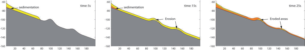

Example of a viscous body sedimenting and eroding with time
See the movie file (980 Ko)

3.1 Pyroclastic flows and pyroclastic surges

A modified version of VolcFlow takes into account two « fluids »: a dense (e.g. block-and-ash flow) and a dilute (ash-cloud surge) fluids.
It allows to simulate ash-cloud surge generated by the dense pyroclastic flows as well as surge-derived flows.

Pyroclastic flows and ash-cloud surge at Merapi volcano

3.2 Simulations of tsunami

A modified version of VolcFlow takes into account two « fluids »: rock avalanche and water. It allows to simulate tsunami generated
by the entrance of a debris avalanche into the see or by coastal destabilization.

Tsunami generated by a submarine destabilization at La Réunion
See the movie file (12.5 Mo)
Read the following paper for further details:
Kelfoun K, Giachetti T, Labazuy Ph, Tsunamis hazard related to major catastrophic collapse at Reunion Island, Submitted J Geophys Res.

Theoretical example of the debris avalanche entering a lake
See the movie file (12.3 Mo)

3.3 Fluidisation

VolcFlow is able to advect the gas pressure and to change the frictions angles according to the pressure.

Comparison between VolcFlow and laboratory experiments (Gueugneau V.))

3.4 Cooling and lava flows

mud flows degasing flow

A variation of the basic version allows advecting any properties. The rheology can depends on these properties.
This allow to calculate the effect of cooling on lava flows and the effect of gaz diffusion on the rheology of granular flows.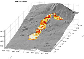

5. Download Examples

These simple examples are done to learn how to use VolcFlow. The users must be able to write programs in Matlab before using VolcFlow.

With the single-fluid version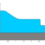

1. Dambreak	2. Collapse A simple collapse on a topography defined by a function	3. Lava flow – how to model a source rate – use of a realistic topography saved in a mat-file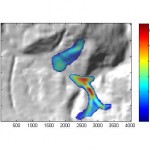
4. Scripts – how to run a series of simulations? – probabilistic analysis – read a Surfer6 file for topography	5. tsunami – how to use an image to define an initial perturbation	6. Concentrated pyroclastic flows
Socompa avalanche (low resolution)

With the two-fluids version: debris avalanche and tsunamis

Download here:

In this example, a 50m-thick avalanche – shaped by the letters of VolcFlow – collapses into the sea.

With the two-fluids version: pyroclastic surge and flow

Download here:

In this example, a retrogressive lava dome collapse forms a pyroclastic flow that creates a pyroclastic surge.

6. Other downloads

Dat-reader file:

These files allow to read data from the .dat file generated by VolcFlow during calculation.
You must modify the file to post-process your data.
Saved variables are defined before the calculation in the input file using the following syntax: saved_var = {‘h’, ‘umx’, ‘umy’};
Download the two files, put them in a same folder and write VF_data_reader in the command window of Matlab.

This section is under construction

Topography files
Files are encoded in Surfer GS-binary Format.You can read them with Matalb using the following instructions :
code = fscanf(fid,’%c’,4)
ncol = fread(fid,1,’int16′)
nlig = fread(fid,1,’int16′)
xmin = fread(fid,1,’float64′)
xmax = fread(fid,1,’float64′)
ymin = fread(fid,1,’float64′)
ymax = fread(fid,1,’float64′)
zmin = fread(fid,1,’float64′)
zmax = fread(fid,1,’float64′)
z = fread(fid,’float32′);z = (reshape(z, ncol, nlig))’;

Conversion vertical geometry / normal geometry
In VolcFlow 1.x.x and 3.x.x, the thickness is defined normal to the ground and not vertically (as in versions 2.x.x).
For debris avalanches and dome collapses, it is often convenient to use DEM differences, which are defined vertically.

This code allows to convert vertical thickness to normal thickness: vertical2normal.m
You can use it in this input file.

This code allows to convert normal thickness to vertical thickness: normal2vertical.m
You can use it to visualize your results.

Calculation of position of the center of mass.

Use these lines to calculate the center of mass of your flows or your deposits:

[I,J]=meshgrid(1:ncol, 1:nrow);
ic = sum(sum(h.*I))./sum(sum(h));
jc = sum(sum(h.*J))./sum(sum(h));
fprintf(‘The center of mass is located in i=%f, j=%f (in meshes).\n’, ic,jc);
%plot(ic*dx_horiz, jc*dy_horiz, ‘*g’)

7. How to use VolcFlow

7.1 Use of VolcFlow

VolcFlow is writen with Matlab and is of very simple use.
Put VolcFlow.p and VolcFlowFig.fig in the same folder.
Type VolcFlow in the command windows and the following figure appears.

Choose the input file, check the result view with « representation » then click ok.
The calculation runs showing the results at each representation time step.

Pause, stop and restart

It could be useful to pause VolcFlow if you need your computer to work with other softwares. Just clic on the « pause » button. To continue, press a key in the commande window.

You can also stop VolcFlow during a calculation.
First, you need to modifiy the inital input file by writing the name of the restart file : restart_file = ‘myrestart.dat’. Then, run VolcFlow as usually.
Three possibilities allows to restart.

1) VF_out.dat
When you stop VolcFlow, a VF_out.dat file is automatically generated. The file contains the basic variables that allow VolcFlow to restart.
It needs a small disk space but it cannot save user-defined variables. You have to rename this file before the next run if you want to conserve it.

2) Workspace
If you use your own variables, complex graphics, records of variables… the best way is to save the workspace of Matlab after VolcFlow stops.
Clic on File and then on Save Workspace as. Then write in the input file : restart_file = ‘myrestart.mat’.
VolcFlow will automatically detect the .mat extension, will load it and will restart exactly as if it was not interupted.
The inconvenient is the large size of the mat-file on the disk.

3) m-file
It is possible to call a external restart m-file. Write in the input file : restart_file = ‘myrestart.m’.
The m-file must call a mat-file. It can be usefull if you need to change some variables of the input file.
Indeed, if you choose to load a workspace, the modifications of the initial input-file (change of the duration of calculation, for example) will be lost.
The structure of the restart m-file is first to load a workspace, then to change variables : tmax = 2000; for example.
Be carreful with this option not to change variables that will cause VolcFlow to become unstable.

7.2 Algorithm

The following image summarizes the algorithm of VolcFlow. It may help the user to write the input file.

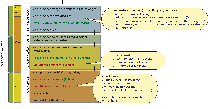
VolcFlow can take into account frictional (with one or two friction angles), viscous, Bingham, Voellmy, etc…as well as user-defined behaviours.
The default equation defining the stress in VolcFlow is :

Where curb is the curbature of the topography in the flow direction.
The terms in blue are to be defined in the input file.
The internal friction (jint or delta_interne in the input file) is used to calculate Kactpass in the constitutive equation:

7.3 Input file

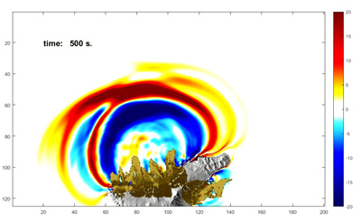
This section shows the input file that must be written to use VolcFlow.
It simulate the flow a an initial mass released to the right and a mass brought at a constant rate to the left. (See the movie file (700 Ko) with a more complex representation).

example of two viscous flows: immediate release (right) and constant rate (left)

Just keep the structure of this file and modify some lines to adapt the input file to the problem you want to solve.
Calculation are always in 2D. To simulated 1D cases, as below, use 3 lines only and the boudary conditions written below.

%This input file allows to simulate a 1D flow
ncol=500;                   %number of rows
nrow = 3;                   %number of lines
dx_horiz = 0.004;           %x space step (m)
dy_horiz = dx_horiz;        %y space step (m)
dt=0.0005;                  %time step (if fixed by the user) in second
tstep_adjust = 0;           %0 = fixed time step, 1 = variable time step defined by VolcFlow
dtplot = 100*dt;            %time step of representation (s)
tmax = 4;                   %time max of calculation (s)
g=9.81;                     % gravity (m.s-2)
delta_int = 0/180*pi;       %internal friction angle (rad)
delta_bed   = 0/180*pi;     %external friction angle (rad)
cohesion =      0;          %threshold (Pa)   
rho = 1000;                 %density (kg.m-3)
coef_u2 =   0;              %u2-resisting force (turbulence or collisional stress)
viscosity = 1;              %viscosity (Pa.s)
%representation  = 'cla; patch([x(1) x x(ncol)],[0 h(2,:)+z(2,:) 0],[0 h(2,:)*0 0],''Facecolor'',[0.5 0.8 1]);
%hold on; patch([x(1) x x(ncol)],[0 z(2,:) 0],[0 h(2,:) 0],''Facecolor'',[0.7 0.7 0.3]); text(0.2,0.2,num2str(t)); axis equal; axis tight;';
representation = 'cla; plot(x, z(2,:)+h(2,:)); hold on;plot(x, z(2,:), ''k''); axis equal '; %representation of results

f_avi =  'c:\example.avi';     %used to produce a movie file during calculation
f_data = 'c:\example.dat';     %used to store the data 

source = 'if t<0.5; h(:,30:60)=h(:,30:60)+0.2*dt; end;';             %source of the model
                   %be carreful: simple condition. Should take into account the momentum conservation
                   %Can also be used to add your own sedimentation laws.

bound_cond = 'h2(1,:)=h2(2,:); h2(nrow,:)=h2(2,:);  ';    %Boudary conditions for 1D calculation

x = [dx_horiz/2:dx_horiz:ncol*dx_horiz-dx_horiz/2];       %Definition of x and y axis. Not necessary.
y = [dy_horiz/2:dy_horiz:nrow*dy_horiz-dy_horiz/2];

z=ones(3,1)*( (x-1.2).^2/2+sin(x*10)/20)+0.2;     %Definition of the topography.
                                                  %It may be either a function or a DEM. z should be a nrow by ncol matrix
                                                 
h(1:nrow, 1:ncol)=0;                              %Definition of the thickness, h should be a nrow by ncol matrix
h(:, 450:480)  = 0.1; 

% initial velocities, defined at the edges of the cells
u_xx(1:nrow, 1:ncol-1)=0;
u_xy(1:nrow, 1:ncol-1)=0;
u_yy(1:nrow-1, 1:ncol)=0;
u_yx(1:nrow-1, 1:ncol)=0;

%other parameters that can be defined
% indCy=[3 5 8];                      %cells were there is no flux. Numerical walls.
% indCx=[12 53 62];
% curvature = 0;                      %1 by default. 0 = the curvature of the topography is not taken into account
% X_Rstress = ''; Y_Rstress = '';     %You can write your own resistive low that can depends on h, u, z ... for example a Pouliquen´s law.
% CFLcond=0.5;                        %By default, the time step is automatically defined (if tstep_adjust == 1) according to the Courant-Friedrich-Levy criterion.
                                      %but it may be lowered to increase the stability. 1 = Courant-Friedrich-Levy criterion, 0.5 = two times lower.
% restart_file = 'VF_out.dat';        %When VolcFlow stops, it generate a VF_out.dat file. It is possible to restart the calculation from the time step VolcFlow stops
                                      %using this line. You may change the name to avoid erasing of VF_out.dat at the next stop.
% doubleUpwind = 0                    %0 by default. 1 = use of a second upwind scheme for momentum adevection. Sometimes more accurate but of a more difficult use.
% uminstop=0;                         %If >0, VolcFlow will stop when the slowest velocity will be slide as a single mass. Usefull to simulate debris avalanches.                                   
t=0; 

7.4 Other features

This section presents various examples to help understanding how to use VolcFlow.

* Script

The use of scripts is usefull to analyse the effect of one or several parameters on the simulation.
The use is presented below:

This file simulate flows of various volumes. Each volume is defined by V in the script file (example_script.m).
V is then used in the source file (source_cond.m) called by the input file (toposcript.m).
At the end, all the areas covered by the flow are stacked to draw a kind of probabilistic hazard map.
Uncompress, define the current directory and type example_script in the command window of Matlab.

When using VolcFlow as a script, the « runs as a script » message appears at the right of the interface window. Below is the number of runs as a script. Close the interface before using VolcFlow in the normal way or write set(findobj(‘tag’,’script’),’string’, ») in the Matlab command window.

* Source conditions

1) how to calculate the momentum conservation at the source?

Write source = ‘source_file;’ in the input file and put the in :

% variation of thickness
dh=h*0;
dh(70:130, 10:50)=0.2*dt./S(70:130, 10:50);

h=h+dh; %new thikness at the centers
dhmx = (dh(:, 2:ncol) + dh(:,1:ncol-1)) / 2; %new thikness at x-edges
dhmy = (dh(2:nrow, 🙂 + dh(1:nrow-1,:)) / 2; %new thikness at y-edges

% momentum cinservation at the edges
u_xx(dhmx>0) = (u_xx(dhmx>0).*hmx(dhmx>0) + 0)./(hmx(dhmx>0)+dhmx(dhmx>0));
u_xy(dhmx>0) = (u_xy(dhmx>0).*hmx(dhmx>0) + 0)./(hmx(dhmx>0)+dhmx(dhmx>0));
u_yx(dhmy>0) = (u_yx(dhmy>0).*hmy(dhmy>0) + 0)./(hmy(dhmy>0)+dhmy(dhmy>0));
u_yy(dhmy>0) = (u_yy(dhmy>0).*hmy(dhmy>0) + 0)./(hmy(dhmy>0)+dhmy(dhmy>0));

see also « a Bingham flow » in the Download section.

2) how to define sedimentation and erosion laws?

* « en masse » sliding

If lA is defined (lA>0 in the input file), the mass is initially forced to slide in a coherent manner.
1) The velocity of each cell, up, is calculated independently
2) The mean velocity, ponderated by the thickness, is then calculated : um = S(up*h) / Sh
3) Finally, the new velocity of each cell is calculated by its previous velocity and the mean velocity: un = up*(1-A) + um*A
where A is defined by A = exp(-t / lA), t being the time.

This allows a decrease of « coherency » with time, following an exponential law.

8. Theory

VolcFlow is based on the depth-average approximation. Using a topography-linked co-ordinate system, with x and y parallel to the local ground surface and hperpendicular to it, the general depth-averaged equations of mass and momentum conservation are:

with:

T = (Tx, Ty) the basal shear stress that depeds on the flow rheology.

VolcFlow can take into account frictional (with one or two friction angles), viscous, Bingham, Voellmy, etc…as well as user-defined behaviours.

The equations were solved using an original shock-capturing numerical method based on a simple or a double upwind Eulerian scheme (fixed by the user). The schemes can handle shocks, rarefaction waves and granular jumps, and are very stable even on complex topography and on both numerically ‘wet’ and ‘dry’ surfaces. (Some numerical schemes require the ground ahead of the avalanche to be covered with a very thin artificial layer of avalanche material: a so-called numerically ‘wet’ surface (Toro, 2001) ).

For the multifluid version, similar set of equations are solve simultaneously, together with interaction laws.

For more details on the equations and the numerical scheme:

Kelfoun K. and T.H. Druitt, 2005, Numerical modelling of the emplacement of the 7500 BP Socompa rock avalanche, Chile. J. Geophys. Res., B12202, doi : 10.1029/2005JB003758, 2005.

Kelfoun K., Giachetti T. and Labazuy P., 2010, Landslide–generated tsunamis at Réunion Island, J. Geophys. Res., Earth Surface, doi:10.1029/2009JF001381.

Kelfoun K., 2011, Suitability of simple rheological laws for the numerical simulation of dense pyroclastic flows and long-runout volcanic avalanches, J. Geophys. Res., Solid Earth, doi:10.1029/ 2010JB007622.

9. Main variables used

zchange 0 = slope calculation is done once, at the beginning
1 = slope calculation is done at each time step. Use it if the topography changes with time

indCx, indCy indices of the cell borders in x and y where the velocity is forced to be null

cohesion cohesion for a Coulomb body or yield strength for a plastic flow (in Pa)

delta_bed basal friction angle for a Coulomb body

delta_int internal friction angle for a Coulomb body

avant_flux expression used to modify the parameters before the flux calculations

bound_cond expression used to define the boundary conditions

ex : bound_cond = ‘h(:,1)=0; h(:,ncol)=0; h(1, :)=0; h(nrow, :)=0;’;

under reconstruction

CFLcond, chemin, coef_C, coef_u2, comptCFL, compteur2, coule, curvature, , dern_conn, doubleUpwind, dt, dtini, dtmax, dtmin, dtplot, dx_horiz, dy_horiz, erosion, f_avi, f_data, fichint, g, h, h_maxvel, hfluxmin, Hmxmin, icone, imageint, imageintR, , kk, lA, nbstepK, ncol, nomfich, nrow, p, pos_icone, pp, print_dt, pw, pz, qr, ratio_uxy, representation, restart_file, rho, Rstress_law, save_step, saved_var, securit, sedimentation, source, t, tmax, tstep_adjust, u, u_xx, u_xy, u_yx, u_yy, uminstop, VFstop, viscosity, vvf, X_Rstress, Y_Rstress, z

10. Tests of the numerical scheme

10.1. Dambreak

In order to check the accuracy of the numerical scheme of VolcFlow you can compare some numerical results with analytical solutions and with simulations based on other numerical schemes.

The first figure shows comparisons between numerical and exact solutions of dam-break problems. The slope is horizontal and there is zero friction. This problem simulates the breakage of a dam separating an initial layer 1.5 m thick (left) from a layer 0.5 m thick (right). The solution reproduces almost exactly the analytical solution, and particularly the frontal shock wave and the thickness of the central plateau.

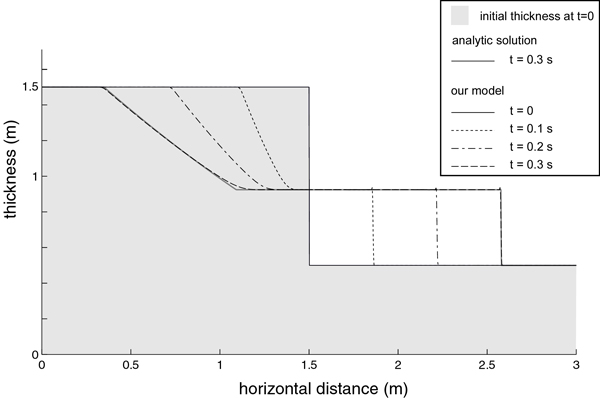
Test of numerical solution against analog solution for a dambreak problem Symetry test of calcultions
See the movie file (230 Ko) See the movie file (750 Ko)

10.2. Granular flow on a slope

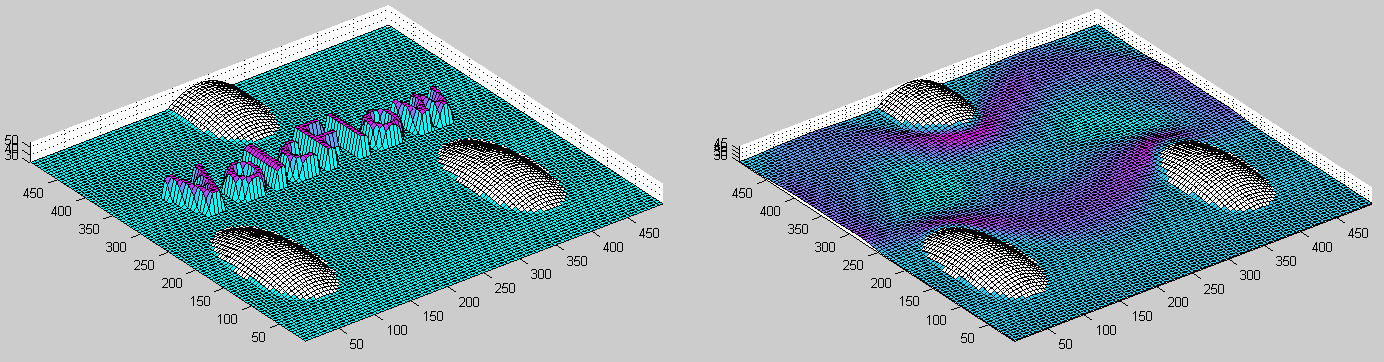
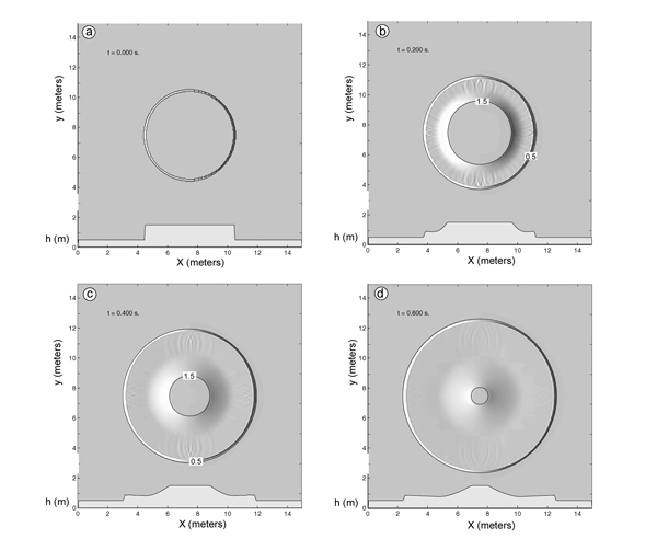
Since the numerical scheme of VolcFlow is based on a rectilinear coordinate system, it is also interesting to perform circular dambreak tests to ensure that the calculations are isotropic.
In the above figure, a 6-m-diameter cylinder of zero-friction fluid, 1.5 m thick, is released onto a 0.5-m-thick, horizontal layer of the same fluid.
The resulting degree of isotropy and shock resolution are both satisfactory, some small numerical oscillations disappearing progressively during the calculation.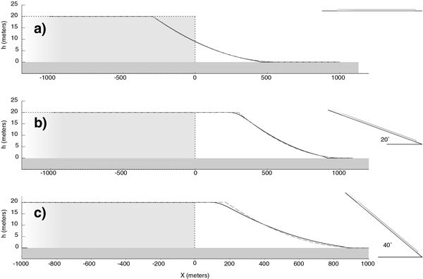

Test of numerical solution against analog solution for a dambreak problem on a slope

Three comparisons with exact solutions obtained by Mangeney et al. (2000) for a dam-break problem on a slope with non-zero friction, and with zero thickness in front of the initial dam. The shape and velocity of the flow are accurately reproduced, even for the least favourable case of a steep slope and high friction angle. Note that the vertical exaggeration of the y-axis exaggerates the difference between numerical and analytical solutions.

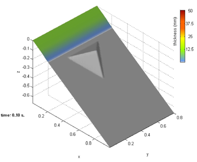
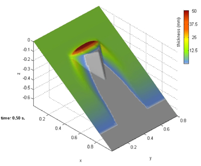
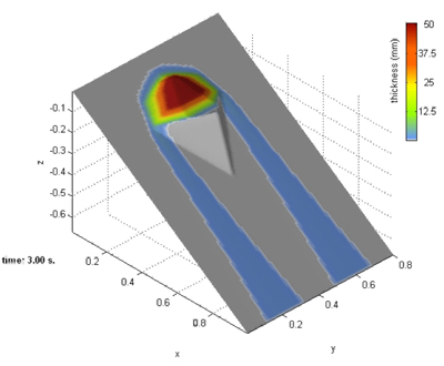
Sand flow (basal friction 32°) on an incline (34°) with a pyramidal obstacle (download the movie file, 2.5 Mo)

10.3. Viscosity

The numerical scheme has been tested independently by Cordonnier et al., 2015.

The benchmark shows a very good accuracy of the numerical scheme of VolcFlow for the simulation of viscous flows.

see B. Cordonnier, E. Lev, and F. Garel, 2015, Benchmarking lava-flow models Geological Society, London, Special Publications, 426, first published on July 10, 2015, doi:10.1144/SP426.7

Known problems with VolcFlow

1. a) You should use the version 2007b or more recent to be compatible withVolcFlow.
2. b) You may receive the following message or wait more than one minute during the initialization phase:
   Java exception occurred
   and […] org.apache.commons.net.ftp.FTP […] solution:
   You should activate your Firewall – http://support.microsoft.com/kb/283673/fr and allow Matlab to accès Internet.
   Without connection, you will be unable to use VolcFlow after 15 days.
3. c) With some computers, 3D views cannot be captured in avi-files. This is due to an incompatibility between Matlab and the graphical capabilities of the computer used.
4. d) VolcFlow works with Microsoft Windows only. I am trying to understand and solve the problème with Linux and McIntosh.